Exploratory data analysis in Scheme
When I started learning Scheme (R6RS), I took the common approach of learning a new language by implementing features from familiar languages (namely R). That approach sent me down the path of writing the dataframe library and porting gnuplot-pipe from Chicken to Chez Scheme. Those two libraries now allow me to conduct simple exploratory data analysis (EDA) in Scheme that should feel relatively familiar to R programmers. In this post, I will work through a simple example, which mostly serves to reinforce how much better suited R is for these types of tasks.
For this post, we will use the Texas housing data included as part of the ggplot2 package for R. I've written that dataset to a CSV file for use in this post. First, let's import the necessary libraries (after following installation instructions in the repos linked above) and then read the data.
(import (dataframe)
        (prefix (gnuplot-pipe) gp:))

> (define df (csv->dataframe "txhousing.csv"))

> (dataframe-display df)

 dim: 8602 rows x 9 cols
     city    year   month   sales    volume  median  listings  inventory       date
    <str>   <num>   <num>   <num>     <num>   <num>     <num>      <num>      <num>
  Abilene   2000.      1.     72.  5.380E+6  71400.      701.     6.3000  2000.0000
  Abilene   2000.      2.     98.  6.505E+6  58700.      746.     6.6000  2000.0833
  Abilene   2000.      3.    130.  9.285E+6  58100.      784.     6.8000  2000.1667
  Abilene   2000.      4.     98.  9.730E+6  68600.      785.     6.9000  2000.2500
  Abilene   2000.      5.    141.  1.059E+7  67300.      794.     6.8000  2000.3333
  Abilene   2000.      6.    156.  1.391E+7  66900.      780.     6.6000  2000.4167
  Abilene   2000.      7.    152.  1.264E+7  73500.      742.     6.2000  2000.5000
  Abilene   2000.      8.    131.  1.071E+7  75000.      765.     6.4000  2000.5833
  Abilene   2000.      9.    104.  7.615E+6  64500.      771.     6.5000  2000.6667
  Abilene   2000.     10.    101.  7.040E+6  59300.      764.     6.6000  2000.7500
Next, we will aggregate the data for plotting to look for annual and seasonal patterns. In Scheme, there is no built-in representation for missing values (like NA in R), but dataframe uses 'na to indicate a missing value. By default, the mean procedure in dataframe removes 'na values.
We will use the same aggregation repeatedly so we will define a custom procedure, df-agg-mod, that applies the same aggregations to different groups. Then, we apply that procedure to df grouped by year.
(define (df-agg-mod df group-names)
  (dataframe-aggregate
    df
    group-names
    '(avg-sales avg-volume avg-median)
    '((sales) (volume) (median))
    (lambda (sales) (exact->inexact (mean sales)))
    (lambda (volume) (exact->inexact (mean volume)))
    (lambda (median) (exact->inexact (mean median)))))

> (define df-agg-year (df-agg-mod df '(year)))

> (dataframe-display df-agg-year)

 dim: 16 rows x 4 cols
    year  avg-sales  avg-volume  avg-median
   <num>      <num>       <num>       <num>
   2000.   478.4581    7.170E+7    96442.00
   2001.   495.6167    7.667E+7   100801.55
   2002.   531.9728    8.571E+7   104365.11
   2003.   539.0849    8.848E+7   108008.28
   2004.   577.2337    9.738E+7   111096.75
   2005.   635.9074    1.138E+8   118384.31
   2006.   664.8815    1.247E+8   124263.48
   2007.   620.6458    1.220E+8   130156.63
   2008.   520.0451    1.019E+8   131297.93
   2009.   469.2169    8.906E+7   131483.76
We can plot data using gnuplot-pipe; a Chez Scheme interface for Gnuplot. I have only a rudimentary understanding of how to use Gnuplot so these plots will be very simple.
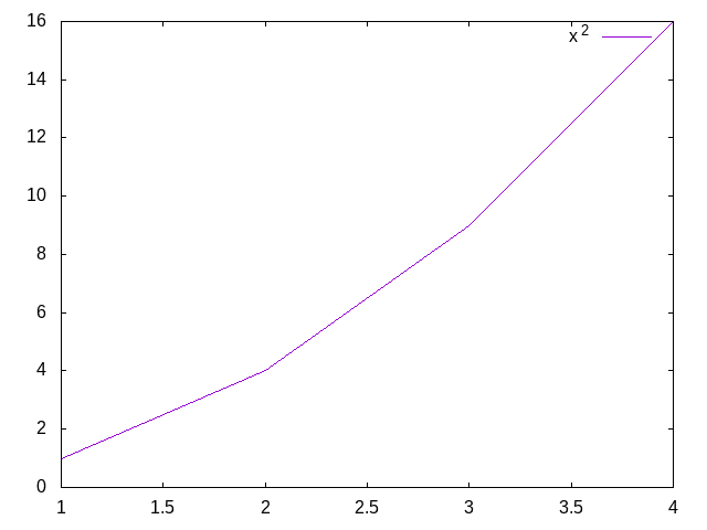
Below is an example of the gnuplot-pipe syntax for a simple line plot. The legend label is followed by lists for the x- and y-values.
(gp:call/gnuplot
 (gp:plot "title 'x^2'" '(1 2 3 4) '(1 4 9 16))
 (gp:save "OneLine.png"))
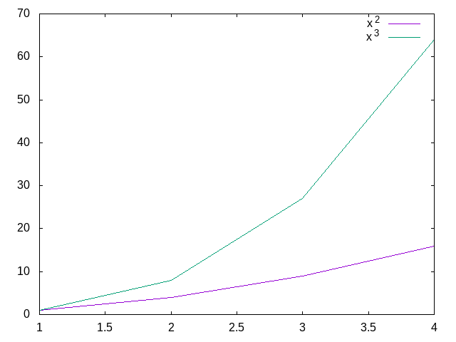
When you want to plot multiple lines, you put the same syntax from the single line plot into a list with each element of the list representing a different line.
(gp:call/gnuplot
 (gp:plot '(("title 'x^2'" (1 2 3 4) (1 4 9 16))
            ("title 'x^3'" (1 2 3 4) (1 8 27 64))))
 (gp:save "TwoLines.png"))
The code for a plot with multiple lines based on a dataframe would be verbose and redundant. We can write a macro to simplify the plotting code. The plot-expr macro takes a dataframe as the 1st argument, x and y column names as the 2nd and 3rd arguments, and the grouping column name as an optional 4th argument. When a grouping argument is specified, plot-expr maps over the unique values in the grouping column to create the list structure expected by gp:plot.
(define-syntax plot-expr
  (syntax-rules ()
    [(_ df x y)
    (list (list "" ($ df (quote x)) ($ df (quote y))))]
    [(_ df x y grp)
     (map (lambda (grp-val)
            (let ([df-sub (dataframe-filter*
                           df
                           (grp)
                           (string=? grp grp-val))])
              (list
               (string-append "title '" grp-val "'")
               ($ df-sub (quote x))
               ($ df-sub (quote y)))))
          (remove-duplicates ($ df (quote grp))))]))
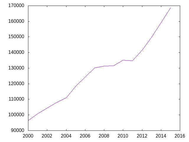
We can now use our plot-expr to plot the data that we aggregated by year across all cities and months. Here we are plotting the average median sale price by year. Nationally, home prices peaked in 2006 and bottomed out in 2012 (source), but, in Texas, housing prices mostly stayed flat during that period.
(gp:call/gnuplot
 (gp:send "unset key")          ; remove legend
 (gp:plot (plot-expr df-agg-year year avg-median))
 (gp:save "MedianSalePriceByYear.png"))
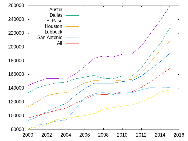
In this next code block, we filter for the selected cities, aggregate by city and year, and then bind the previously aggregated dataframe, df-agg-year, while adding a city column to df-agg-year with the value of All in every row. We created a city-filter because it will be used again below.
(define city-filter
  (lambda (city)
    (member city '("Austin" "Dallas" "El Paso" "Houston" "Lubbock" "San Antonio"))))

(define df-agg-city-year
  (->  df
       (dataframe-filter '(city) city-filter)
       (df-agg-mod '(city year))
       (dataframe-bind
        (dataframe-modify*
         df-agg-year
         (city () "All")))))
The next plot includes 7 lines, but the plot-expr is mostly the same as for plotting one line.
(gp:call/gnuplot
 (gp:send "set key top left")
 (gp:plot (plot-expr df-agg-city-year year avg-median city))
 (gp:save "MedianSalePriceByYearAndCity.png"))
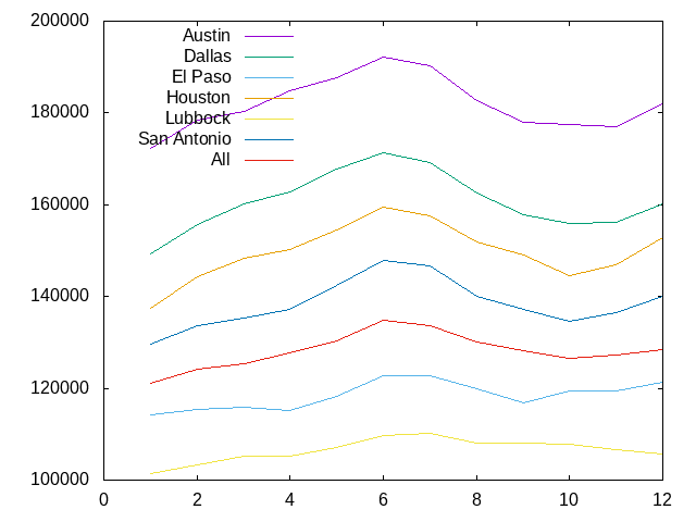
The code is very similar for monthly patterns.
(define df-agg-month
  (-> df
      (df-agg-mod '(month))
      (dataframe-sort* (< month))))

(define df-agg-city-month
  (->  df
       (dataframe-filter '(city) city-filter)
       (df-agg-mod '(city month))
       (dataframe-sort* (< month))
       (dataframe-bind
        (dataframe-modify*
         df-agg-month
         (city () "All")))))

(gp:call/gnuplot
 (gp:send "set key top left")
 (gp:plot (plot-expr df-agg-city-month month avg-median city))
 (gp:save "MedianSalePriceByMonthAndCity.png"))
In conclusion, it's been fun to see that something I built is moderately useful for exploratory data analysis, but it would be a HUGE amount of work to take these libraries to a place where it could even partially replace R for me. To be clear, I wasn't trying to replace R. I was just learning Scheme.